
Machine learning vs. Abrams, Bolomey and Feret: a fair test on 28-day strength
We cross-validated the three classical strength laws against machine learning on 425 lab specimens at 28 days. Machine learning is more accurate where it has data, and its limits point to physics-informed AI.
- concrete
- compressive strength
- machine learning
- physics-informed AI
- mix design
Every concrete engineer learns Abrams’ law early, and most of us still use it, or one of its relatives, every week. When someone claims that a machine learning model predicts strength better, the reaction in a lab or a technical department is usually polite skepticism. That skepticism is healthy. Most published comparisons use small datasets, random train/test splits that leak information, and metrics reported without the conditions behind them.
So I ran the comparison myself, on a public dataset, with a protocol designed to be hard on the machine learning side. This article shows what came out, including the case where machine learning does worse. My conclusion is that machine learning is clearly the more accurate tool for 28-day strength when it has data from a comparable mix space, and that its remaining weakness is exactly where physics has the most to offer.
The data and the question
The dataset is the well-known concrete compressive strength set published by I-Cheng Yeh (1998): laboratory mixes with cement, blast furnace slag, fly ash, water, superplasticizer, coarse and fine aggregate, and the measured strength at a given age. I kept only the 28-day results: 425 specimens from 417 distinct mixes, with strengths from about 8 to 82 MPa.
The question is simple: given a mix design, how well can each approach predict its 28-day compressive strength on mixes it has not seen?
The contenders
Classical laws. All three are fitted by nonlinear least squares, with the same inputs:
- Abrams: f = A / B^(w/b)
- Bolomey: f = K (b/w − a)
- Feret: f = K [V_b / (V_b + V_w + V_a)]², with absolute volumes and entrapped air fixed at 20 L/m³
In their original form these laws only see cement. That is unfair in a dataset where 81% of the 28-day mixes contain slag or fly ash. On the full dataset, using cement alone costs the laws 2 to 6 MPa of RMSE. So I gave them an effective binder, b = C + k_s·S + k_f·F, with the efficiency factors k_s and k_f fitted from the data. This is the strongest version of the classical approach I could build without changing its physics. On the full 28-day set, Abrams gives A = 131 MPa, B = 11.3, k_s = 0.74 and k_f = 0.40, values that a materials engineer will find reasonable.
Machine learning. A linear regression on the seven ingredients (as a sanity baseline), gradient-boosted trees, and a Gaussian process (GP) with one length scale per ingredient. None of them is told anything about water-to-binder ratio or hydration. They only see the seven quantities in kg/m³.
Physics-informed. A model that combines a classical strength law with machine learning, included as a reference point for the discussion at the end of this article.
How the test was run
Three choices matter more than the choice of algorithm.
- Split by mix, not by row. Repeated specimens of the same mix always stay on the same side of the split. Otherwise the model is graded partly on mixes it has already seen.
- Refit everything inside each fold. The k-factors of the laws and the hyperparameters of the ML models are learned on the training fold only.
- Report the spread. 10-fold cross-validation repeated 5 times, with RMSE, MAE and R² on predictions the models never trained on.
Result 1: with data from a comparable mix space, machine learning is more accurate
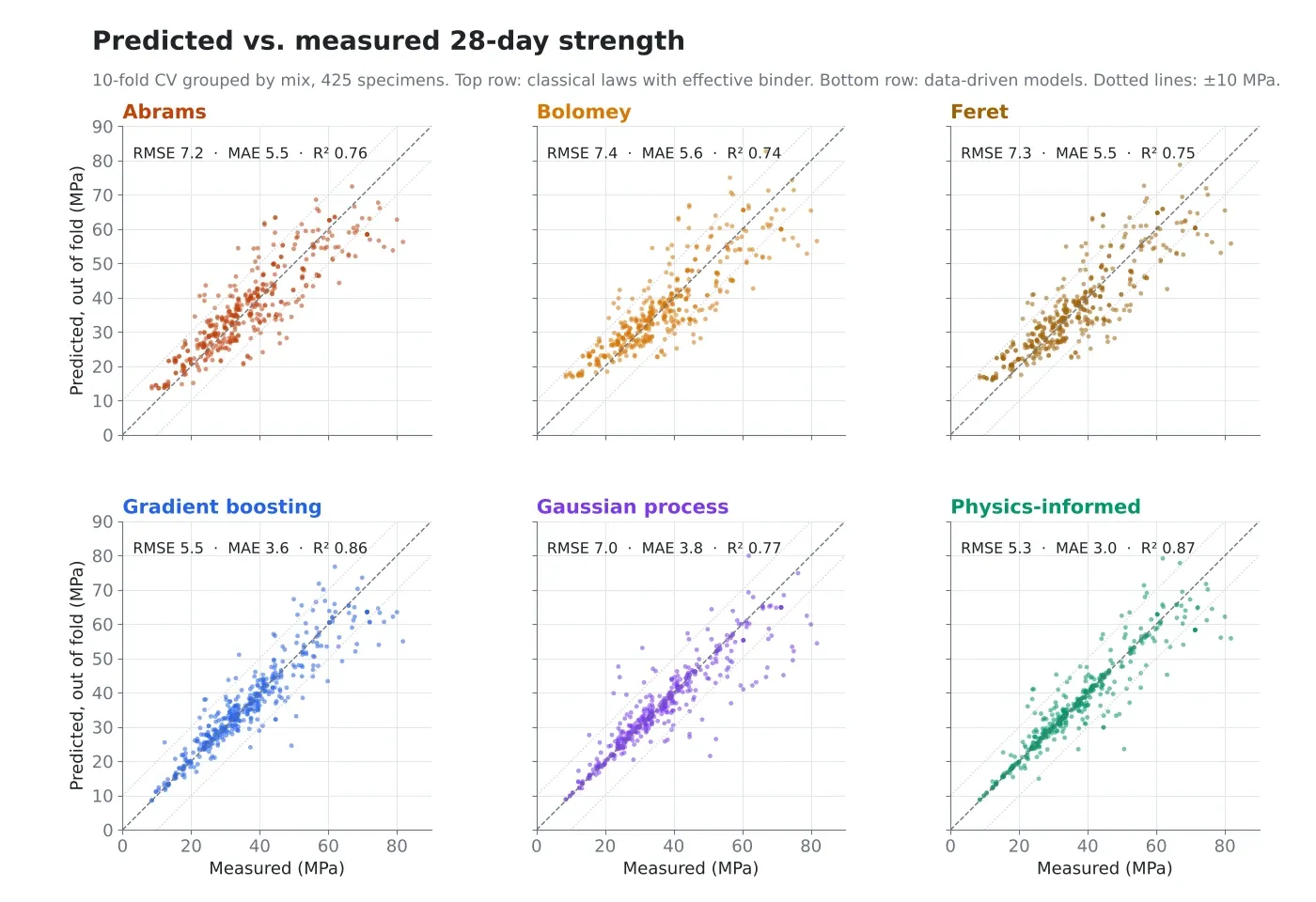
Figure 1. Out-of-fold predicted vs. measured 28-day strength, one point per specimen. Dotted lines mark ±10 MPa. Linear regression is in the table only.
| Model | RMSE (MPa) | MAE (MPa) | R² |
|---|---|---|---|
| Abrams, effective binder | 7.19 | 5.45 | 0.76 |
| Feret, effective binder | 7.29 | 5.48 | 0.75 |
| Bolomey, effective binder | 7.44 | 5.60 | 0.74 |
| Linear regression | 7.21 | 5.40 | 0.76 |
| Gaussian process | 6.96 ± 0.50 | 3.85 | 0.78 |
| Gradient boosting | 5.54 | 3.56 | 0.86 |
| Physics-informed | 5.31 ± 0.31 | 3.01 | 0.87 |
10-fold CV grouped by mix, mean of 5 repeats. The ± is the standard deviation across repeats, shown where it exceeds 0.2 MPa.
Four observations.
First, the three laws are practically equivalent once they share an effective binder. The spread between them is 0.25 MPa. They are also no better than a plain linear regression on the ingredients. Their limit is not the choice between Abrams, Feret or Bolomey. It is the shared structure: strength as a function of one ratio, water to binder (or binder to voids), plus two efficiency factors. Superplasticizer dosage, aggregate content and the interaction between slag and fly ash have no place in the equation.
Second, gradient boosting reduces RMSE by 23% compared with the best law, from 7.2 to 5.5 MPa, and the typical error (MAE) by about a third, from 5.5 to 3.6 MPa. R² goes from 0.76 to 0.86. For a producer, that is the difference between a trial batch that confirms the design and one that has to be repeated.
Third, the Gaussian process is the most instructive case. Its MAE is 30% lower than Abrams, so on most mixes it is much more accurate. Its RMSE, however, is barely better and varies between repeats. On a few mixes far from the rest of the data it misses badly, because a purely data-driven model with no prior knowledge returns to the average strength of the training set when it has no close neighbors. Keep this behavior in mind for the second result.
Fourth, the physics-informed model is the most accurate of all: RMSE 5.3 MPa and MAE 3.0 MPa, 45% below the typical error of the best law.
Result 2: outside the training range, physics keeps its advantage
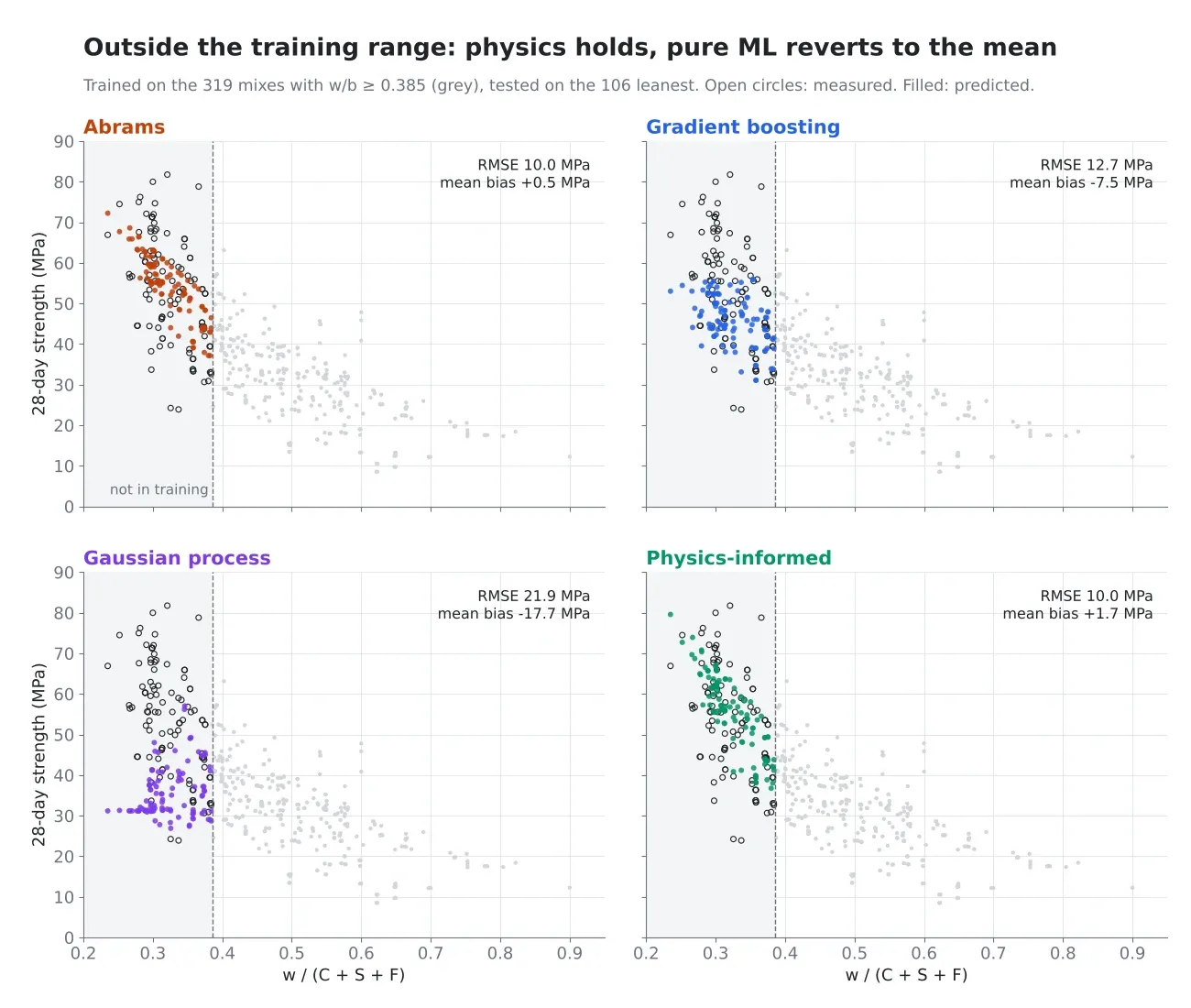
Figure 2. Models trained only on mixes with w/b ≥ 0.385, then asked to predict the 106 leanest mixes. Measured strengths in this region average 53.5 MPa, while the strongest training mix reached 63 MPa.
A fair article has to include the test where machine learning loses. I trained every model on the 319 mixes with a water-to-binder ratio of 0.385 or higher, and asked them to predict the 106 mixes below it. This is a real situation: a producer who has mostly made ordinary concrete and now wants to design a high-strength mix.
| Model | RMSE (MPa) | Mean bias (MPa) |
|---|---|---|
| Abrams | 9.97 | +0.5 |
| Linear regression | 9.93 | +2.2 |
| Physics-informed | 10.00 | +1.7 |
| Feret | 10.10 | +1.8 |
| Bolomey | 11.97 | +5.6 |
| Gradient boosting | 12.65 | −7.5 |
| Gaussian process | 21.89 | −17.7 |
Abrams extrapolates with almost no bias, because the exponential dependence on w/b is physics, not a fit to the training range. Gradient boosting cannot predict above the strengths it has seen and underestimates by 7.5 MPa on average. The GP falls back to the mean strength of the training set (about 31 MPa) and underestimates by almost 18 MPa. None of these failures would be visible in a standard cross-validation.
The physics-informed model stays with the classical laws here, at 10.0 MPa with a small bias. It is the only model in this study that is both the most accurate on familiar mixes and as reliable as the laws on unfamiliar ones.
What this means in practice
For skeptical readers, this is how I would summarize the evidence:
- On 28-day strength, machine learning is more accurate than the classical laws when it has a few hundred results from a comparable mix space. Here gradient boosting gains 23% in RMSE and about a third in typical error over the best law, measured on mixes the models never saw, with a protocol that penalizes leakage.
- The classical laws are not wrong, they are incomplete. They capture the dominant mechanism and they extrapolate well. They cannot learn the second-order effects that make the difference in a real plant: admixture dosage, aggregate content, SCM interactions.
- Pure machine learning can fail silently outside its data. Its errors on unfamiliar mixes are large and biased, and a standard validation does not reveal them. Any tool that recommends new mixes has to address this, because new mixes are exactly what you want to explore.
- Combining both removes the trade-off, at least on this dataset. The physics-informed model is the most accurate on familiar mixes and does not lose the robustness of the laws on unfamiliar ones.
Opening the discussion: physics-informed AI
The weakness of pure machine learning is the strength of the classical laws. That is not a coincidence, and it suggests the next question is not “physics or machine learning”, but how to build models that carry both.
Physics-informed AI is the general name for this idea. The knowledge the profession has accumulated over a century is given to the model instead of being rediscovered from data. A strength law is only the simplest example. Monotonic constraints (more water should not increase strength, all else equal), hydration kinetics and the maturity concept for age, packing models for the aggregate skeleton, and the chemistry of supplementary cementitious materials can all be built in. The potential follows from the results above. Such models should become useful with fewer results, because they do not start from zero. They should behave sensibly outside their data, because their default is physics, not the dataset average. And they should stay interpretable, because their parameters keep a physical meaning that an engineer can check.
There are open questions, and they deserve debate. Which physics is reliable enough to impose as a hard constraint, and which should only be a soft prior? How do we handle cements, aggregates and admixtures that change from one plant to another? How much uncertainty should a model report before its recommendation for a new mix is trusted?
This is the direction we are working on at Alfraido: data-efficient models fitted on each producer’s own results, grounded in the physics of cement and concrete rather than replacing it, and explicit about their uncertainty.
I would welcome the discussion, especially with those who doubt it. Which physical knowledge would you insist on seeing in such a model before you trusted it with a new mix?
Method notes and reproducibility
- Data: I-Cheng Yeh, “Modeling of strength of high performance concrete using artificial neural networks,” Cement and Concrete Research 28(12), 1797–1808 (1998). Dataset © Prof. I-Cheng Yeh, UCI Machine Learning Repository. 28-day subset only.
- Laws: fitted by bounded nonlinear least squares with five starting points per fit; k_s and k_f bounded to [0, 1.5]. Feret uses specific gravities of 3.15, 2.90 and 2.30 for cement, slag and fly ash.
- Gaussian process: standardized inputs, squared-exponential kernel with one length scale per ingredient plus white noise, normalized target, hyperparameters by maximum marginal likelihood.
- Gradient boosting: histogram-based trees, 500 iterations, learning rate 0.05, 15 leaves, minimum 5 samples per leaf.
- Validation: grouped 10-fold CV by mix, 5 repeats; extrapolation split at the 25th percentile of w/(C + S + F). All models, including the physics-informed one, are refitted on the training data only.
- Limits: one dataset, from one laboratory program, without cement chemistry, aggregate properties or curing variations. The ranking between models should be checked on plant data before it is generalized.